Diffusion net notes
Key physical ideas:
- diffusion models are continuous storages that use heat equations for search in high-dimensional space
- search is performed via image cooling, building storage is done via reversed process
- sampling techniques can be studied from perspective of school physics thermal process like adiabatic, isothermal and more
Many ideas in top papers can be derived from school physics, which are hard to be seen due to complex terminology 😔. Hope that will help you in your research and experiments.
Introduction
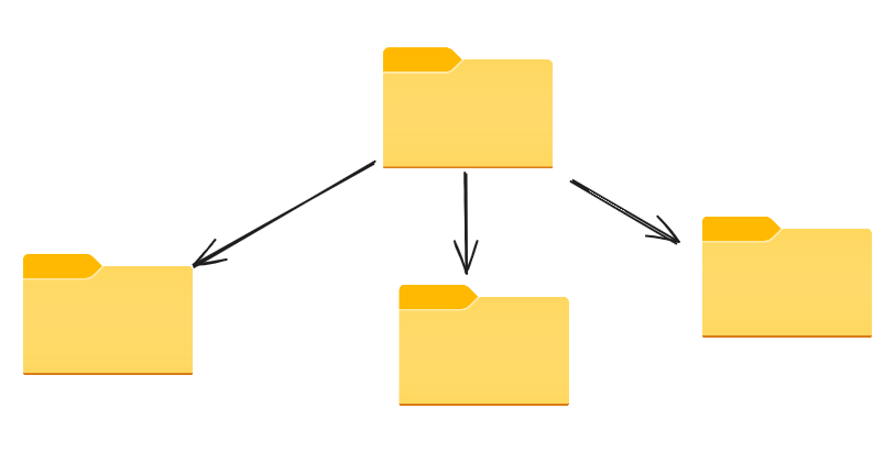
File systems are organized hierachicallly. It helps to preserve context and hasten search
 |
|---|
| File storage provides way of information organization |
But happens if wants to do continuate hierarchy. How it will look like, what properties will it have?
Physics matter
In computer science methods using energy are called energy-based and are mostly popularized via Yann LeCun.
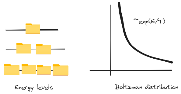
In physics concept of continuous hierarchy comes naturally from observation of energy spectre of gas \(p(E) = \frac{exp(-\frac{E}{T})}{Z}\)
Distribution is called Boltzman and explains probability of particle. You may argue how probability refers to files. So I’ll share distribution of files under energy.
 |
|---|
| Continious file storage |
See, exponent in probability perfectly matches with idea in hierarchy on every level number of files should grow, therefore we will observe.
Terminology
In section we will refer to physics terminology, which may seem more familiar as their corresponds to nature. I have prepared some beautiful pictures for you to guide through main concepts of temperature, free energy and gaussian noise.
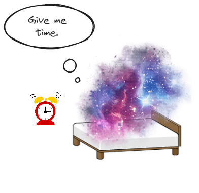
Temperature
Temperature gives average energy of particle in system by simple equation
\(E = d/2 T\) ,where $d$ is a dimension of space and $T$ is temperature.
Cold is training pictures, hot is initial gaussian. Let’s see how temperature varies distribution
 |
|---|
| High temperature corresponds allows more states |
Free energy
$Z$ in normalization is tightly connected with concept of Free energy. In layman terms is maximal energy that you can get from battery considering lack of thermal energy.
Physict write
\[F = U - TS\],where $U$ is inner energy, $S$ - entropy, $T $-temperature of system. Informally, it’s a gap between ordered - potential and unordered - kinetic energy.
Fundamental principle of universe is minimization of this gap.
 |
|---|
| Universe is quite lazy. It tends to minimize free energy |
This concept although comes in motion, where it has a representation of Lagrangian
\[L = T - V\]This principle is crucial in bayessian optimization and model selection.
By the way so called KL-divergence is actually a free energy 🤯.
Gaussian noise is hierarchical
The most important thing about gaussian, that it’s rescales. If you average random gaussian variables you’ll again get gaussian, but at greater scale
\(\sum \xi \sim \mathbf{N}(0,N), \xi \sim \mathbf{N}(0,1)\) That’s it gaussian noise is hierarchical properties as it seamlessly accumulate information from is ancestors.
 |
|---|
| Even noise can build hierarchy |
And help her a lot with our noise task
What actually happens through denoising process?
This chapter gradually steps from concept of file storage to diffusion nets. Explains concepts of locality
Process
Network learns gradually to correct mistakes. This is great explanation, but intuition for building your own approach.
Let’s recall main diffusion equation
\[{\displaystyle x_{t}={\sqrt {1-\beta _{t}}}x_{t-1}+{\sqrt {\beta _{t}}}z_{t}}\]See $\beta$ in diffusion is reverse temperature $\frac{1}{T}$ and we’ll built intuition why it is useful
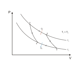
I argue that this process is actually a thermal cycle
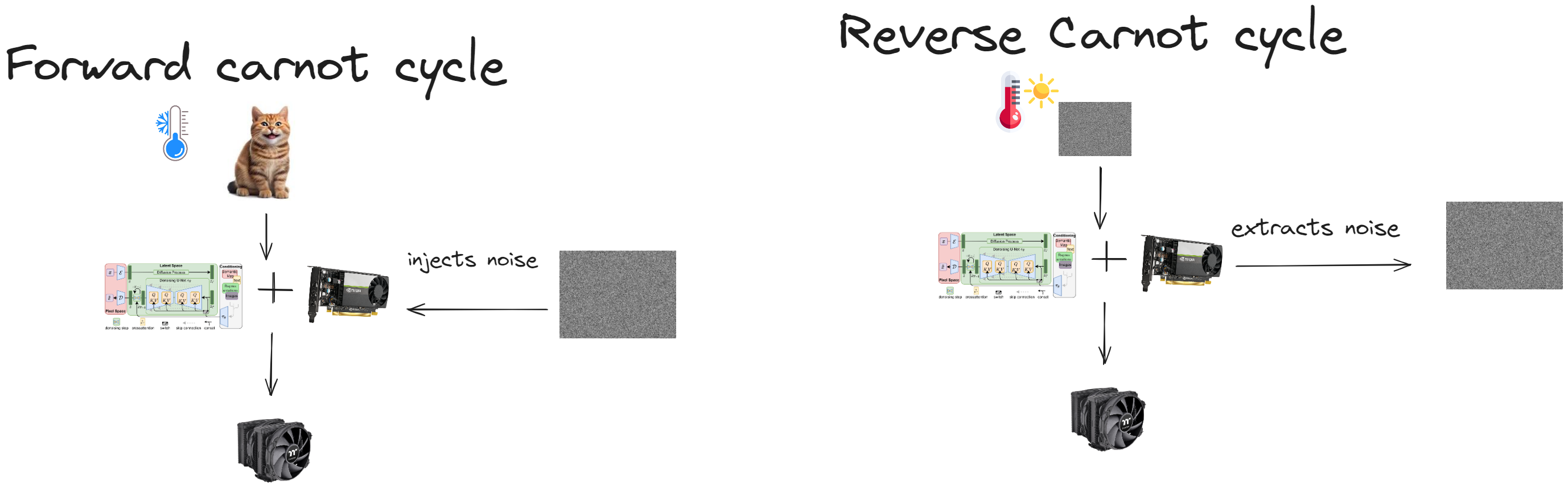 |
|---|
| *Kolmogorow writes describes thermal process. Can you estimate if energy conversion efficiency $\eta$ :)? * |
But how it’s possible? I mean GPU heats when train. Yeah refrigiator of cooler does it too 🤯. But then he transverse heat to atmosphere, so it can grab heat again. It’s called reverse carnot cycle
One more suggestion before me may build theory. Diffusion build similarity of objects based on their similarity in more.
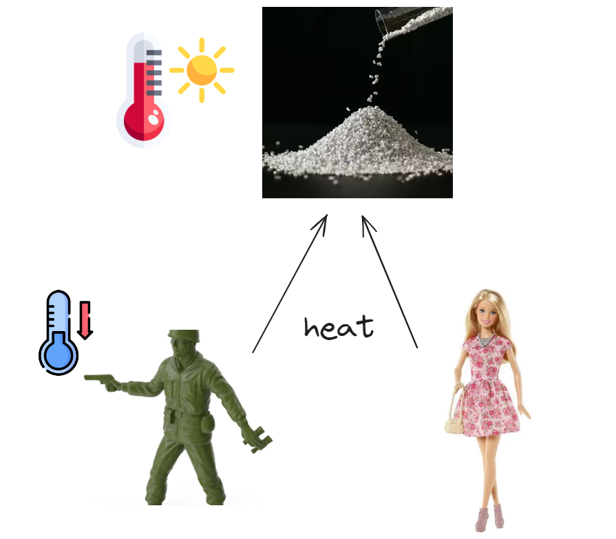 |
|---|
| You want to know something similar. Hmm.. just heat it |
So, what is actually happening, through forward process is a heating of images to build hierarchy based on similarity.
 |
|---|
| Distribution hierarchy |
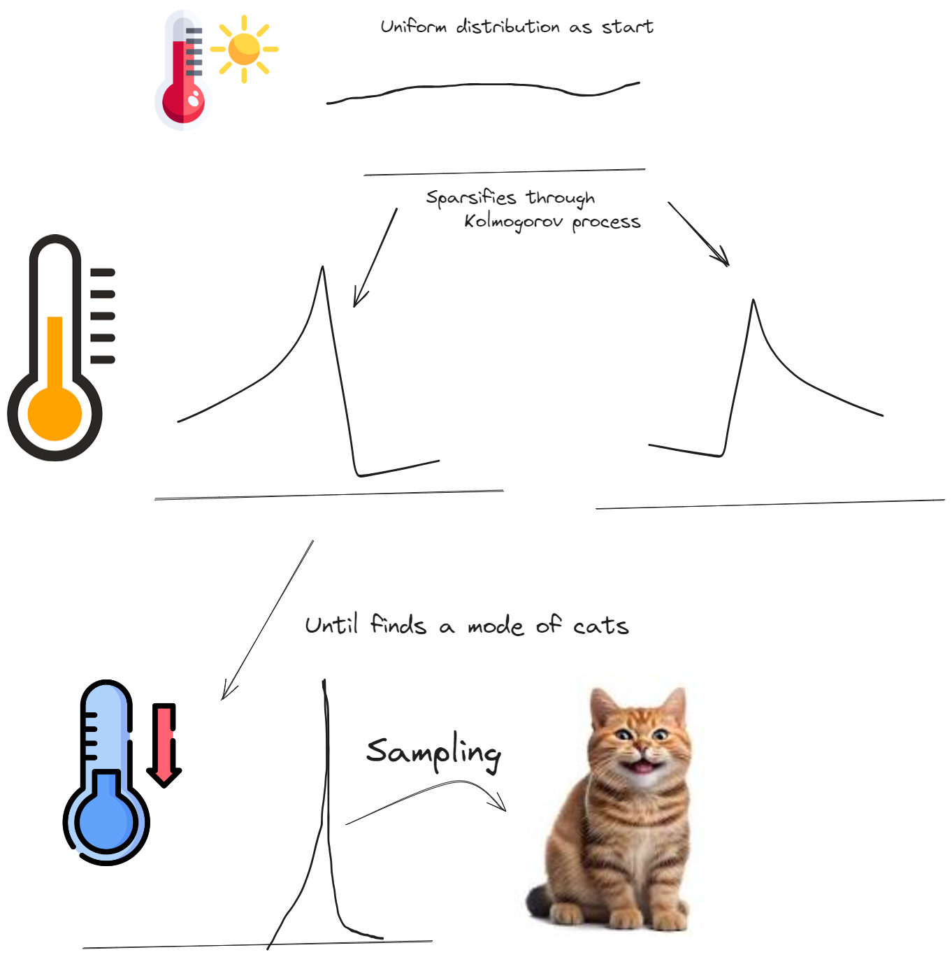
What’s more temperature naturally sets scale of
How that happens?
It happens through local minimization of local free energy on manifold. Free energy is a metric of best cataloging of whole manifold, score function is it’s local gradient.
\[score = - \frac{\partial F}{x}\]That’s it by minimization of score you build perfect catalogue and your diffusion net know have map. That means that recataloging is done locally. Starting from shelfs
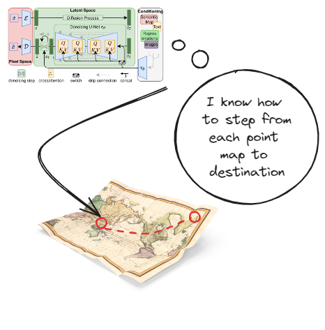 |
|---|
| Map shows direction on where step further from all point |
So that diffusion can effectively catalog all info from pictures. Every step is recataloging info in best format possible. Actually it means that net builds geodesics on manifold.
How net understand direction?
For understanding let’s write small distortion of distribution in energy using Taylor series :
\[q(E + \Delta E) = q(E) + \nabla_E q(E) \Delta E\]For energy based gradient can be derived as
\[p(E) = \frac{exp(-\frac{E}{T})}{Z} \\ \nabla_E p = - \frac{exp(-\frac{E}{T})}{Z \cdot T} \\\]So that relation between probabilities of distorted and undistorted energy levels is given by:
\[\frac{q(E+\Delta E)}{q(E)} = 1 - \Delta E /T\]Note that relation between levels doesn’t depend on current energy! Hierarchy order depends only on temperature. This property is important is at it brings continuous symmetry of translation in corresponding algebra.
Direction is built from gradient of $\nabla_x \ln q_x$, which in literature is noted as score.
Following scores builds shortest path from one point to another on manifold. Yet geodesic may not always desirable.
Recall train loss of diffusion net:
\[\sum_{t=1}^T KL(q(x_{t-1}|x_t,x_0) \| p_\theta(x_{t-1}|x_t))\]It is hard to ascertain what that loss means. Let’s build intuition with placing book in library. When you walk you need to find a department, than case, shelter and finally a place. For that case we will have T=4 and each term corresponds for task of searching.
 |
|---|
| Diffusion does it on every hierarchy level |
Note that
Note that every process is decomposed. You can train on any task to be better in whole. This decomposition idea, was introduced in simpler loss
\[\mathrm{E}_{t,\epsilon_t\sim N(0,1), x_0}\left[\|\epsilon_t - \epsilon_\theta (\sqrt{\bar{\alpha}} x_0 + \sqrt{1-\bar{\alpha}}\epsilon_t)\|^2\right]\]Don’t be messed with brackets. $\sqrt{\bar{\alpha}} x_0 + \sqrt{1-\bar{\alpha}}\epsilon_t$ is an argument of $\epsilon_\theta$, which to corresponds to neural net prediction.
Notice that “simple” equation is overcomplicated with discrete timestamps. Physics perspective doesn’t restrict special spaces.
You can model sampling techniques as thermal process
Euler sampling is isothermal as it brings equal portions of heat on each step.
Why we need neural nets?
Because their are very good at learning continuous symmetries. Therefore they are great in interpolating, which is great property for
You can learn about symmetries from my other blog.
Conclusions
I’ll provide you key bullets
- training set is cold 🥶, original noise is very hot 🥵
- diffusion iteratively cools 🧊 source noise
- it trains to do that via heating 🔥
- you can use school physics to study diffusion
See, you can even build optimal diffusion through Carno cycle.
 |
|---|
| Optimal cycle for cooling and heating |
It’s very interesting, if it is possible to measure
##
Related themes
Here some themes that are tightly related, but I am still strugling to wrench them to article
Fokker-Plank equation through flux
\[\frac{\partial}{\partial t} p(x,t) = - \frac{\partial}{\partial x}[\mu(x,t)p(x,t)] + \frac{\partial^2 p(x,t)}{\partial x^2}\]Corresponding diffusion shift can rewriten $\mu(x,t)= \mu(x)$ can be reduced to potential of gradient $V(x)$.
Rearranging derivatives in right side brings noition of flux
\[\frac{\partial}{\partial x}\left[\frac{\partial V(x)}{\partial x} p(x)+ \frac{\partial{p(x)}}{\partial x}\right] = \frac{\partial}{\partial x} J(x)\]Through sampling in Langevin dynamics we bring flux through diffusion term. Recall
\[dX_t = \underbrace{-\nabla V(X) dt}_{\text{drift term}} +\underbrace{\sqrt{2} dB_t}_{\text{diffusion term}}\]Stationary distribution with $\frac{\partial p(x,t)}{\partial t} = 0$ brings:
\[\frac{\partial p(x,t)}{\partial t} = \frac{\partial J(x)}{\partial x} = 0\]Which can rewritten as:
\[\\]Solution is formed in: \(p(x) \sim exp(-V(x))\)
Note that stationary distirbution in thermal system is hierarchical.
Quantum perspective
Energy level are actually discrete, but are expanded through brownian motion of particles.
Normal distribution. Information geometry approach
It can be shown that riemanian metric of gaussian distribution is equal to: \(g = \frac{1}{\sigma^2}(d\mu^2+2d\sigma^2)\)
That speculations is very important due to fact it’s curvature defines hyperbolic space as them naturally hierarchical
Diffusion maps
Is approach for dimension reduction similar as PCA and t-SNE. You can read more
Connection to optimal transport
Yandex research paper
Two steps:
- Transforming ODE to probability flow ODE
- Encoder map For a given distribution µ0 and a timestep t, let us denote the flow generated by this vector field as Eµ0 (t, ·). I.e., a point x ∼ µ0 is mapped to Eµ0 (t, x) when transported along the vector field for a time t. The ‘final’ encoding map is obtained when t → ∞, i.e,
Note that $E_{\mu_0}$ implicitly depends on all the intermediate densities µt obtained from the diffusion process (or the Fokker-Planck equation).
The authors of Meng et al. (2021) proposed to view diffusion models as a discretization of certain stochastic differential equations. SDEs generalize standard ordinary differential equations (ODEs) by injecting random noise into dynamics. Specifically, the diffusion process specified by Equation (1) is a discretization of the following SDE:
\[dx = -\frac{1}{2} \beta(t) xdt + \sqrt{\beta(t)} d\omega\]r. It can be shown that the trajectory {µt}∞ t=0, obtained by solving the Fokker-Planck equation
Useful resources
Blogs:
- Markov chains https://bjlkeng.io/posts/markov-chain-monte-carlo-mcmc-and-the-metropolis-hastings-algorithm/
Videos:
- https://www.youtube.com/watch?v=hbIfrLefwzw